---
author: "Louis-Philippe Caron and Núria Pérez-Zanón"
date: "`r Sys.Date()`"
output: rmarkdown::html_vignette
vignette: >
%\VignetteEngine{knitr::knitr}
%\VignetteIndexEntry{Most Likely Tercile}
%\usepackage[utf8]{inputenc}
---
Most Likely Tercile
========================
This vignette aims to illustrate a step-by-step example of how to determine the most likely tercile of a forecast using CSTools functionalities.
### 1- Required packages
The functions to compute the Weather Regimes are part of CSTools while plotting functions are included in s2dverification package:
```r
library(CSTools)
library(s2dverification)
library(easyVerification)
library(multiApply)
library(CSTools)
require(zeallot)
```
### 2 - We define 2 functions
#### A function to produce our terciles
```r
quantile_aux = function(data, n_categories = 3){
data = as.vector(data)
q = quantile(x = data, probs = 1:(n_categories - 1) / n_categories, type = 8, na.rm = TRUE)
return(q)
}
```
#### A function to convert the continuous ensemble forecast to counts of ensemble members per category
```r
c2p <- function(forecast, t) {
colMeans(easyVerification::convert2prob(as.vector(forecast), threshold = as.vector(t)))
}
```
### 3 - We define the region to look at
```r
lat_min = 25
lat_max = 52
lon_min = -10
lon_max = 40
```
### 4 - We define the start dates for the hindcasts/forecast (in this case, May 1st 1981-2020) and create a sequence of dates.
```r
ini <- 1981
fin <- 2020
numyears <- fin - ini +1
mth = '05'
start <- as.Date(paste(ini, mth, "01", sep = ""), "%Y%m%d")
end <- as.Date(paste(fin, mth, "01", sep = ""), "%Y%m%d")
dateseq <- format(seq(start, end, by = "year"), "%Y%m%d")
```
### 5 - We define a target season: JJA.
```r
mon1 <- 2
monf <- 4
```
### 6 - Finally, we define the model, the reference, the variable of interest and the common grid.
```r
forecastsys <- 'system5c3s'
obs <- 'erainterim'
grid <- "256x128"
clim_var = 'tas'
```
### 7 - We load the data.
```r
c(exp,obs) %<-% CST_Load(var = clim_var, exp = forecastsys,
obs = obs, sdates = dateseq, leadtimemin = mon1, leadtimemax = monf,
lonmin = lon_min, lonmax = lon_max, latmin = lat_min, latmax = lat_max,
storefreq = "monthly", sampleperiod = 1, nmember = 10,
output = "lonlat", method = "bilinear",
grid = paste("r", grid, sep = ""))
```
### 8 - We extract the latitude and longitude of the data.
```r
Lat <- exp$lat
Lon <- exp$lon
```
#
### 9 - We extract the anomalies from the forecasts and the observations.
```r
c(ano_exp, ano_obs) %<-% CST_Anomaly(exp = exp, obs = obs, cross = TRUE, memb = TRUE)
```
### 10 - We compute the seasonal mean of forecasts and observations.
```r
ano_exp$data <- Mean1Dim(ano_exp$data,4)
ano_obs$data <- Mean1Dim(ano_obs$data,4)
```
### 11 - We create our terciles using Apply.
```r
quantiles <- multiApply::Apply(data = ano_exp$data, target_dims = c('sdate','member'),
quantile_aux, output_dims = 'bin', ncores = 4)$output1
```
### 12 - We calculate the probability using Apply and c2p.
```r
probs <- Apply(data = list(forecast = ano_exp$data, t = quantiles),
target_dims = list('member', c('bin')), #, 'member')),
fun = c2p, output_dims = 'bin', ncores = 4)$output1
```
### 13 - We extract the data for the latest forecast.
```r
prob_map <- drop(probs)[,numyears,,]
names(dim(prob_map)) <- c('bin','lat','lon')
```
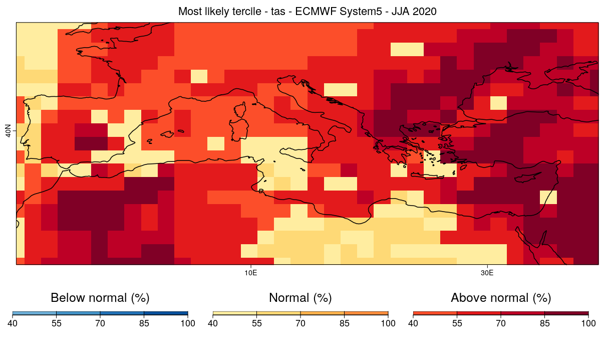
### 14 - We plot the most likely quantile.
```
CSTools::PlotMostLikelyQuantileMap(probs = prob_map, lon = Lon, lat = Lat,coast_width=1.5, legend_scale = 0.8,
toptitle = paste0('Most likely tercile - ',variable,' - ECMWF System5 - JJA 2020'),
width = 12, height = 7, fileout = paste0(clim_var, '_most_likely_tercile.png'))
```
 #
### We can also mask the regions for which the model doesn't have skill. For this, we will calculate the RPSS and exclude the region for which the value is smaller or equal to 0.
### 15 - First, we evaluate the RPSS, i.e. the skill at predicting the right tercile.
```r
v2 <- aperm(drop(ano_obs$data),c(3,2,1))
v2 <- v2[,,1:(numyears-2)]
v1 <- aperm(drop(ano_exp$data),c(4,3,2,1))
v1 <- v1[,,1:(numyears-2),]
RPSS <- veriApply('FairRpss',fcst=v1,obs=v2,ensdim=4,tdim=3,prob =c(1/3,2/3))
```
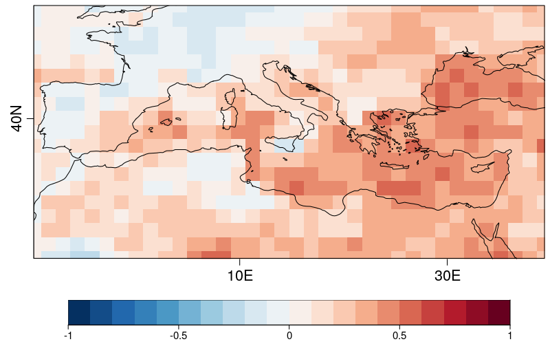
### 16 - We can plot the RPSS.
```r
PlotEquiMap(RPSS[[1]], lat=Lat,lon=Lon, brks=seq(-1,1,by=0.1),filled.continents=F,
fileout = paste0(figures_path, clim_var, '_RPSS.png'))
```
#
### We can also mask the regions for which the model doesn't have skill. For this, we will calculate the RPSS and exclude the region for which the value is smaller or equal to 0.
### 15 - First, we evaluate the RPSS, i.e. the skill at predicting the right tercile.
```r
v2 <- aperm(drop(ano_obs$data),c(3,2,1))
v2 <- v2[,,1:(numyears-2)]
v1 <- aperm(drop(ano_exp$data),c(4,3,2,1))
v1 <- v1[,,1:(numyears-2),]
RPSS <- veriApply('FairRpss',fcst=v1,obs=v2,ensdim=4,tdim=3,prob =c(1/3,2/3))
```
### 16 - We can plot the RPSS.
```r
PlotEquiMap(RPSS[[1]], lat=Lat,lon=Lon, brks=seq(-1,1,by=0.1),filled.continents=F,
fileout = paste0(figures_path, clim_var, '_RPSS.png'))
```
 ### 17 - From the RPSS, we create a mask. Regions with RPSS<=0 will be masked.
```r
mask_rpss <- RPSS[[1]]
mask_rpss[RPSS[[1]] <= 0] <- 1
mask_rpss[is.na(RPSS[[1]])] <- 1
mask_rpss[RPSS[[1]] > 0] <- 0
```
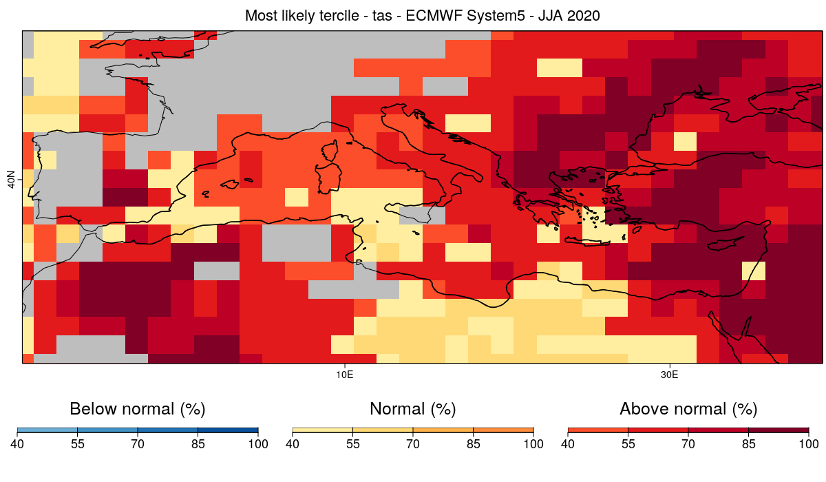
### 18 - Finally, we plot the latest forecast using the mask.
```r
CSTools::PlotMostLikelyQuantileMap(probs = prob_map, lon = Lon, lat = Lat,coast_width=1.5, legend_scale = 0.8,
mask = t(mask_rpss),
toptitle = paste0('Most likely tercile - ',variable,' - ECMWF System5 - JJA 2020'),
width = 12, height = 7,
fileout = paste0(clim_var, '_most_likely_tercile_mask.png'))
```
### 17 - From the RPSS, we create a mask. Regions with RPSS<=0 will be masked.
```r
mask_rpss <- RPSS[[1]]
mask_rpss[RPSS[[1]] <= 0] <- 1
mask_rpss[is.na(RPSS[[1]])] <- 1
mask_rpss[RPSS[[1]] > 0] <- 0
```
### 18 - Finally, we plot the latest forecast using the mask.
```r
CSTools::PlotMostLikelyQuantileMap(probs = prob_map, lon = Lon, lat = Lat,coast_width=1.5, legend_scale = 0.8,
mask = t(mask_rpss),
toptitle = paste0('Most likely tercile - ',variable,' - ECMWF System5 - JJA 2020'),
width = 12, height = 7,
fileout = paste0(clim_var, '_most_likely_tercile_mask.png'))
```