
Sidebar
This is an old revision of the document!
Table of Contents
Universal Kriging - Urban Group
Context
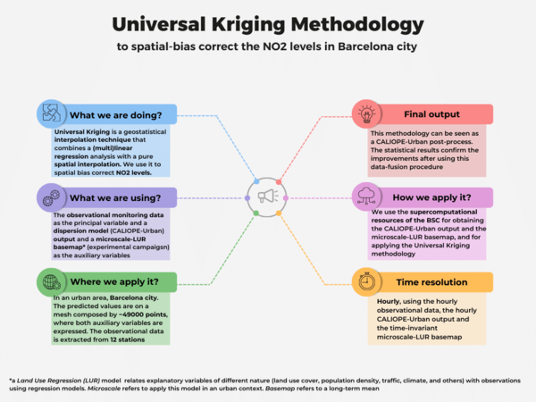
Universal Kriging is a common geostatistic technique used for spatial interpolation, that combines a (multi)linear regression analysis —with auxiliary variables called covariates— along with a spatial interpolation —done taking into account the auto-correlated spatial structure of the data—. In our case, we have applied this methodology as a post-process of the CALIOPE-Urban dispersion model, developed by the Earth Science Department of the Barcelona Supercomputing Center (BSC). To implement it, we have used the hourly observational NO2 data coming from 12 monitoring stations as the principal variable, and the CALIOPE-Urban hourly NO2 output as the covariate. In addition, we have studied the added value to incorporate as the second covariate our time-invariant microscale-Land Use Regression (LUR) model, developed by using two different NO2 passive dosimeters campaigns and 8 predictors (urban geometric variables, simulated vehicular traffic densities, annually-averaged data bi-linearly interpolated from the regional CALIOPE system and the annually-averaged NO2 output of CALIOPE-Urban) through a machine learning approach. Our implementation is a data-fusion procedure used as a spatial NO2 bias correction in an urban area, the city of Barcelona. Moreover, this correction can be applied directly to the daily maximum NO2 concentrations, instead of the hourly levels. For more information, suggestions or clarifications, please do not hesitate to write an email to the Authors. Notice that a new paper about the implementation of this methodology is under revision.
Authors
Álvaro Criado Romero, alvaro.criado@bsc.es
Jan Mateu Armengol, jan.mateu@bsc.es
Meriem Hajji, meriem.hajji@bsc.es
First Steps
To follow a basic tutorial using this methodology, please follow the next steps. The procedure is implemented using the R software.
Using the GitLab repository and copying all the needed archives
- Copy all the functions and archives needed to implement the procedure in your own directory. To do that, open a terminal and copy the following command:
git clone https://earth.bsc.es/gitlab/es/universalkriging.git
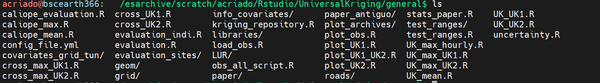
After doing that, a folder called by default universalkriging will appear with all the copied files from the repository: https://earth.bsc.es/gitlab/es/universalkriging.git. This will be the main folder, which contains the sub-folder general (the one with all scripts and data), and there the results will appear. All of this information will be mentioned again in the following steps.
After copying that repository, a list of different archives will appear. They are classified into R scripts (the principal script is named by kriging_repository.R , while the remaining R scripts are secondary scripts called by the principal one in different parts of the workflow), folders (they contain different types of information, required for some of the mentioned scripts), a configuration file (named by config_file.yml , used by initializing the methodology and launching it in terms of what procedure we would want, as it can be seen in the next steps) and git-basic files (as, the README.md).
At this point, I recommend following the tutorial using the Rstudio program to visualize the different scripts.
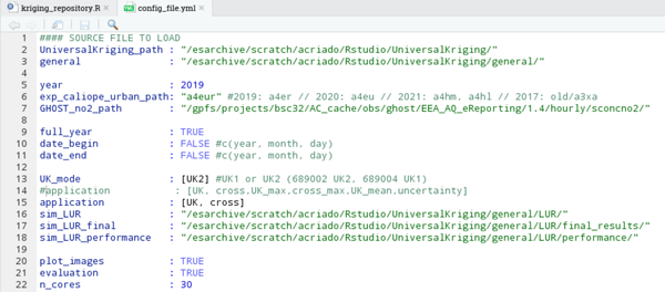
The configuration file
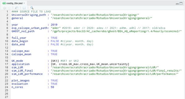
The configuration file is an archive used as a setup structure, which means that the variables that appear in it can be changed and it will produce a different output. It is a separate file, so the main advantage is that can be modified without varying the rest of the scripts. The first step to begin consists of filling it. Notice that this is the only archive that has to be modified in terms of your goal. Before starting to modify it, its shape would look like this:
- Through the Rstudio visualization:
- Through the terminal. To do that, go to the directory where all archives copied from the repository are kept, and type the following (in this case, the visualization is done through the program MobaXterm):
vi config_file.yml
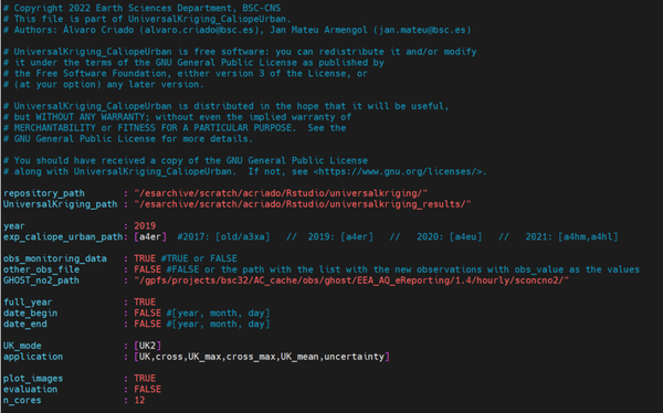
Now we are going to see what is and the implication of each of the items that have to be filled in the configuration file:
- UniversalKriging_path : (a folder path)
this will be the main folder. In the begging, it must contain the folder with all the archives copied from the above repository, which would be general:- general : (a folder path)
this path must be the one where all the archives copied from the repository are kept, and it is included in the UniversalKriging_path.
- year : (a number)
this is referred to the choosen year. The available years are 2017, 2019, 2020 and 2021.- exp_caliope_urban_path : (a character). Each character refers to an experiment, depending on the chosen year (2017: old/a3xa ; 2019: a4er ; 2020: a4eu ; 2021: a4hm, a4hl).
This parameter is needed in order to use the CALIOPE-Urban output linked to the year of application. In the first application, the output is copied into the user's directory from one of the experiments mentioned. The user only should fill the character in terms of the chosen year, but the experiments should be the mentioned ones if the correct version of CALIOPE-Urban will be used. This has to be written between “”. - GHOST_no2_path : (a folder path: “/gpfs/projects/bsc32/AC_cache/obs/ghost/EEA_AQ_eReporting/1.4/hourly/sconcno2/”)
this is the path needed to use the observations coming from the monitoring stations used. In the first application, the observations will be copied into the user's directory from that path. The user should not change this path if the GHOST observations will be used.
- full_year : (TRUE or FALSE)
if the user wants to bias-correct the whole year, this parameter would be TRUE, then date_begin and date_end will be FALSE. If full_year is FALSE, the period chosen cannot involve two different years. In other cases:- date_begin & date_end : (R-vector format: c(year, month, day) )
if full_year is FALSE, the user has to fill this parameter as a vector of R that contains the year, month and day to begin the methodology.
- UK_mode : (UK1 or UK2)
this parameter is referred to the usage or not of the microscale-LUR model as the second covariate. If UK_mode is UK1, only CALIOPE-Urban is used as the covariate. If UK_mode is UK2, both CALIOPE-Urban and the microscale-LUR model will be the covariates. This has to be written between [ ]. Only if the UK_mode is UK2 the microscale-LUR model will be used, but the following paths have to be filled in any case:- sim_LUR : (a folder path)
this is the path that contains all the information about our microscale-LUR model. This path must be referred to the folder LUR copied from the repository, kept in the general folder. For example, if the general path is /esarchive/scratch/acriado/UniversalKriging/general/ , the sim_LUR path would be /esarchive/scratch/acriado/UniversalKriging/general/LUR/ same as ~/general/LUR/. * sim_LUR_final : (a folder path)
this is the path that contains the information about the final microscale-LUR basemap. The folder LUR already includes this folder, so the user has to refer to it from that path. This folder is called final_results (path: ~/general/LUR/final_results). * sim_LUR_performance : (a folder path)
this is the path that contains the information about the expected performance of the microscale-LUR basemap. The folder LUR already includes this folder, so the user has to refer to it from that path. This folder is called performance (path: ~/general/LUR/performance) . * application : (all possible combination using the following items; UK, cross , UK_max, cross_max, UK_mean, uncertainty )
this is referred to the application of the methodology that we want. This/They has/have to be written between [ ]: * UK: Universal Kriging hourly correction (the default). * cross: If we want to apply the Leave-One-Out Cross-Validation, and get the results only at the monitoring stations. * UK_max and cross_max: They are the same, as mentioned before, but instead of the hourly application, the daily maximum one. * UK_mean: Is for computing the daily mean and annual mean corrected concentrations. If the UK application is not performed before applying this, nothing will occur. * uncertainty is for calculating the daily mean variances, the annual mean variance and the relative uncertainty associated with the application. * plot_images : (TRUE or FALSE)
if TRUE, plots are generated. * evaluation : (TRUE or FALSE)
if TRUE, a statistical evaluation is performed * n_cores : (a number)
it is referred to the cores of the machine requested to submit the job. The applications are parallelized in terms of the day. It means that, for instance, the spatial bias correction of the 29/03/2019 is done at the same time than the 30/03/2019 one. In the section The main scriot and its explanation or Submitting Jobs we give an idea to choose this number. As a resume, notice that the user only has to do the following about the configuration file: * Choosing its own UniversalKriging_path and referring to it the paths general, sim_LUR, sim_LUR_final and sim_LUR_performance. * Choosing one of the years available, with the appropriate exp_caliope_urban_path, and choosing between a whole year correction or not. * Choosing the Universal Kriging mode in terms of the covariates, the application, if plotting and doing the evaluation or not and the cores to submit the job. * (The rest of the configuration should not be changed, only fill it as is explained). === The structure of the folders === Before applying the methodology and obtaining the results, is important to realize the structure of the folders that will appear to understand correctly the different outputs. The structure of the folders created by the code is always the same, and it is constructed at the first moment after applying any of the possible applications, which means some folders may be empty. Some specifications of the folders will be addressed in the next steps, following the workflow of the code. This is an example of the structure using the 2019 dataset :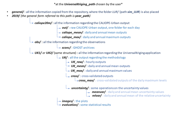 Remember that the parallelization is carried out in terms of the day. We are applying the methodology on a mesh composed approximately of 49000 points, each hour of the period chosen. The output of this methodology is daily, which means that the output files are referred to each day. Thus, each file will contain the correction on the 49000 points, 24 times regarding the 24h of the day. Please, see the examples to visualize the outputs of this methodology.
=== The main script and its explanation ===
The kriging_repository.R script, placed in the folder general, is the main script regarding the application of the methodology and the one that is going to be submitted. Please, open it to see the code and the following explanation (through Rstudio or the terminal, the same as the visualization of the configuration file). Notice that the user does not have to change this script, the only part ready to change is the configuration file. It is split into different sections:
* The first section, Config file, is about setting up the procedure by reading the configuration file.
* The section initial setting takes into account:
- The principal libraries that are going to be used and the coordinates reference.
- The pollutant, in this case we have to type NO2 and no2 for the model and observations configurations respectively.
- The variogram's optimization, basically if changing or not the variogram model parameters.
- The parameter paper, if TRUE some specific operations are made for the paper that we are made about this methodology.
* In the section initial setting: directories, the folders structure explained above is created in the UniversalKriging_path given the configuration chosen.
* In the section initial setting: variables:
- All regarding dates is being set up.
- The mesh where the bias correction takes place and the observational sites are introduced. The mesh is the same as the CALIOPE-Urban one, composed of approximately 49000 points.
* In the section observations, a script is used regarding reading the observations, preparing their format, etc.
* In the section caliope evaluation, mean and max, different scripts are used to prepare the files regarding the model (CALIOPE-Urban) output at the monitoring stations (caliope evaluation), and computing the mean and maximum daily and annual values.
* In the section variogram total, the variogram and its model are created.
* The section covariates is only used if the UK_mode is UK2, since refers to the microscale-LUR model. Two different scripts (sim_LUR_final & sim_LUR_performance) are employed to address its expected performance and the basemap, respectively.
* In the section application, all the applications established by the user are made.
* In the section plots, the images are generated if the configuration's parameter plot_images is TRUE. The same for the section evaluation, where the specific operations about the paper are made if the parameter paper of the initial setting section of the current script is set to TRUE.
Notice that the majority of the secondary operations —for example preparing the observations or extracting the CALIOPE-Urban annual mean— are made in the first application of the user. It means that if the user wants to apply another configuration file, keeping the same period of time, and still using the same paths configuration, the corresponding files are already created based on another previous application and the secondary operations are not computed again. For this reason, a stable folder structure is made and documented. For example, 6h of computational time using 50 cores are needed to calculate the daily mean concentrations of CALIOPE-Urban for a whole year, which implies that those operations, along with the daily maximum ones, will require approximately 12 hours of computation in the first submission, but not for a second application.
=== Submitting jobs ===
*It is recommended to first take a look at the guidelines of the machines (NORD3v2 or Marenostrum4 -MN4- specifically) to familiarize yourself with this environment (url: https://www.bsc.es/user-support/nord3v2.php ).
To apply the methodology, a job has to be submitted using the supercomputacional resources of the BSC. To do so, a file [name].sh has to be prepared, taking into account the guidelines established in the user's guides of the BSC machines. In the examples, the machine NORD3v2 is the employed one. We recommend the following computational times regarding job directives:
* #SBATCH –time=48:00:00 : if the user wants to apply for the first time (the secondary operations are not made yet) a whole year correction using all the applications available, with approximately between 30 and 50 cores for the parallelization. In this case, due to the high number of computational requirements of the job, we also recommend constraining the memory to “high” : #SBATCH –constraint=highmem. For example, the calculation of the daily mean values of caliope urban during a whole year takes 6h of computational time using 50 cores.
* #SBATCH –time=01:00:00 : if the user wants to apply, without secondary operations and during a whole year, the applications of UK and cross, with approximately 30 cores for the parallelization.
To submit the job regarding this methodology, the user only has to launch its own [name].sh archive with the Rscript kriging_repository.R followed by the configuration file. As an example:
<code bash>
#!/bin/bash
#SBATCH –job-name=“kriging”
#SBATCH –output=K_%j.out
#SBATCH –error=K_%j.err
#SBATCH –time=01:00:00
#SBATCH –qos=bsc_es
#SBATCH -n 30
module load R
Rscript /esarchive/scratch/acriado/Rstudio/UniversalKriging/general/kriging_repository.R /esarchive/scratch/acriado/Rstudio/UniversalKriging/general/config_file.yml
</code>
===== Examples =====
In the following examples, the UniversalKriging_path is :
Remember that the parallelization is carried out in terms of the day. We are applying the methodology on a mesh composed approximately of 49000 points, each hour of the period chosen. The output of this methodology is daily, which means that the output files are referred to each day. Thus, each file will contain the correction on the 49000 points, 24 times regarding the 24h of the day. Please, see the examples to visualize the outputs of this methodology.
=== The main script and its explanation ===
The kriging_repository.R script, placed in the folder general, is the main script regarding the application of the methodology and the one that is going to be submitted. Please, open it to see the code and the following explanation (through Rstudio or the terminal, the same as the visualization of the configuration file). Notice that the user does not have to change this script, the only part ready to change is the configuration file. It is split into different sections:
* The first section, Config file, is about setting up the procedure by reading the configuration file.
* The section initial setting takes into account:
- The principal libraries that are going to be used and the coordinates reference.
- The pollutant, in this case we have to type NO2 and no2 for the model and observations configurations respectively.
- The variogram's optimization, basically if changing or not the variogram model parameters.
- The parameter paper, if TRUE some specific operations are made for the paper that we are made about this methodology.
* In the section initial setting: directories, the folders structure explained above is created in the UniversalKriging_path given the configuration chosen.
* In the section initial setting: variables:
- All regarding dates is being set up.
- The mesh where the bias correction takes place and the observational sites are introduced. The mesh is the same as the CALIOPE-Urban one, composed of approximately 49000 points.
* In the section observations, a script is used regarding reading the observations, preparing their format, etc.
* In the section caliope evaluation, mean and max, different scripts are used to prepare the files regarding the model (CALIOPE-Urban) output at the monitoring stations (caliope evaluation), and computing the mean and maximum daily and annual values.
* In the section variogram total, the variogram and its model are created.
* The section covariates is only used if the UK_mode is UK2, since refers to the microscale-LUR model. Two different scripts (sim_LUR_final & sim_LUR_performance) are employed to address its expected performance and the basemap, respectively.
* In the section application, all the applications established by the user are made.
* In the section plots, the images are generated if the configuration's parameter plot_images is TRUE. The same for the section evaluation, where the specific operations about the paper are made if the parameter paper of the initial setting section of the current script is set to TRUE.
Notice that the majority of the secondary operations —for example preparing the observations or extracting the CALIOPE-Urban annual mean— are made in the first application of the user. It means that if the user wants to apply another configuration file, keeping the same period of time, and still using the same paths configuration, the corresponding files are already created based on another previous application and the secondary operations are not computed again. For this reason, a stable folder structure is made and documented. For example, 6h of computational time using 50 cores are needed to calculate the daily mean concentrations of CALIOPE-Urban for a whole year, which implies that those operations, along with the daily maximum ones, will require approximately 12 hours of computation in the first submission, but not for a second application.
=== Submitting jobs ===
*It is recommended to first take a look at the guidelines of the machines (NORD3v2 or Marenostrum4 -MN4- specifically) to familiarize yourself with this environment (url: https://www.bsc.es/user-support/nord3v2.php ).
To apply the methodology, a job has to be submitted using the supercomputacional resources of the BSC. To do so, a file [name].sh has to be prepared, taking into account the guidelines established in the user's guides of the BSC machines. In the examples, the machine NORD3v2 is the employed one. We recommend the following computational times regarding job directives:
* #SBATCH –time=48:00:00 : if the user wants to apply for the first time (the secondary operations are not made yet) a whole year correction using all the applications available, with approximately between 30 and 50 cores for the parallelization. In this case, due to the high number of computational requirements of the job, we also recommend constraining the memory to “high” : #SBATCH –constraint=highmem. For example, the calculation of the daily mean values of caliope urban during a whole year takes 6h of computational time using 50 cores.
* #SBATCH –time=01:00:00 : if the user wants to apply, without secondary operations and during a whole year, the applications of UK and cross, with approximately 30 cores for the parallelization.
To submit the job regarding this methodology, the user only has to launch its own [name].sh archive with the Rscript kriging_repository.R followed by the configuration file. As an example:
<code bash>
#!/bin/bash
#SBATCH –job-name=“kriging”
#SBATCH –output=K_%j.out
#SBATCH –error=K_%j.err
#SBATCH –time=01:00:00
#SBATCH –qos=bsc_es
#SBATCH -n 30
module load R
Rscript /esarchive/scratch/acriado/Rstudio/UniversalKriging/general/kriging_repository.R /esarchive/scratch/acriado/Rstudio/UniversalKriging/general/config_file.yml
</code>
===== Examples =====
In the following examples, the UniversalKriging_path is :
/esarchive/scratch/acriado/Rstudio/UniversalKriging/ . This is the shape of the directories UniversalKriging/ and general/ before applying the methodology: * UniversalKriging_path * The general path
 ==== Universal Kriging using CALIOPE-Urban as the unique covariate and the whole 2019 data, using all the possible applications ====
- Preparing the configuration file: in this case the same as the example above.
- Enter the machine:
<code bash>
ssh bscXXXXX@nord4.bsc.es
+——————————————————————————+
| |
| .-.–_ |
| ,´,´.´ `. |
| | | | BSC | |
| `.`.`. _ .´ |
| `·`·· |
| |
| |
| _ _ _ _ _ |
| | \ | |/ \| \| \_ \ | \ |
| | \| | | | | |) | | | |) |_ ) | |
| | . ` | | | | _ /| | | | <\ \ / / |
==== Universal Kriging using CALIOPE-Urban as the unique covariate and the whole 2019 data, using all the possible applications ====
- Preparing the configuration file: in this case the same as the example above.
- Enter the machine:
<code bash>
ssh bscXXXXX@nord4.bsc.es
+——————————————————————————+
| |
| .-.–_ |
| ,´,´.´ `. |
| | | | BSC | |
| `.`.`. _ .´ |
| `·`·· |
| |
| |
| _ _ _ _ _ |
| | \ | |/ \| \| \_ \ | \ |
| | \| | | | | |) | | | |) |_ ) | |
| | . ` | | | | _ /| | | | <\ \ / / |
| | |\ | || | | \ \| || |) |\ V /_ |
| |_| \_|\/|_| \_\_// \_/|| |
| |
| |
| |
| |
| - Welcome to Nord3v2!! This machine has the same architecture as Nord3 |
| but with updated OS and Slurm! |
| |
| OS Version: Red Hat Enterprise Linux 8.4 (Ootpa) |
| Slurm version: slurm 21.08.8-2 |
| |
| |
| Please contact support@bsc.es for further questions |
| |
+——————————————————————————+
</code>
3. Preparing the job: the sh file is called by kriging_repository.sh. The user has to write the job directories needed to submit it, as the guidelines specificate. The job directories required in this case would be:
* #SBATCH –job-name : the job's name
* #SBATCH –output : the name of the job's output file
* #SBATCH –error : the name of the job's error file
* #SBATCH –qos : the queue chosen to submit the job. It is related to the cores and the computational time
* #SBATCH –time : the computational time required
* #SBATCH -n : the machine's nodes required
* #SBATCH –constraint : if memory options are required, highmem to high resources, medmem to medium-capacity resources. If memory options are not required, the user should not type this option.
As it would be the first submitted job, we use the maximum computational time (48h) and in this case, we choose to use 50 cores. The queue has to be bsc_es in this case.
<code bash>
#!/bin/bash
#SBATCH –job-name=“kriging_first”
#SBATCH –output=K_f_%j.out
#SBATCH –error=K_f_%j.err
#SBATCH –time=48:00:00
#SBATCH –qos=bsc_es
#SBATCH -n 50
#SBATCH –constraint=highmem
module load R
Rscript /esarchive/scratch/acriado/Rstudio/UniversalKriging/general/kriging_repository.R /esarchive/scratch/acriado/Rstudio/UniversalKriging/general/config_file.yml
</code>
4. Submitting the job. With the configuration file and the job prepared, the user just has to submit the job:
<code bash>
sbatch kriging_repository.sh
</code>
5. If the user types:
<code bash>
squeue
</code>
is possible to see the status of the job. The fields that appear are:
* JOBID: ID identification of the job.
* PARTITION: machine's specification.
* NAME: the name of the job.
* USER: the user's number.
* ST: the status of the job, first if it is pending (PD) or running (R). Other options are completed (CD), completing (CG), failed (F), preempted (PR), suspended (S) or stopped (ST). All of this can be seen in the machine's guidelines.
* TIME: the time that has passed since the job is running.
* NODES: the machine's nodes required for the job. It is related to the cores chosen.
* NODELIST(REASON): machine's specification.
This is an example, in this case the directory where the job is launched is / esarchive/scratch/acriado/nord3/ :
 6. Waiting until the job is finished. Notice that when a job is submitted, two files are created: the output and the error ones (the user has defined their names in the job directories). In the output file, the user can visualize some indications that appear while running the job. In the error one, the user can see secondary errors that maybe were not enough to cancel the job's running as well as the error if the job was stopped.
7. The job is completed. A folder named by 2019/ will be created at the Universalkriging_path, with the same folder structure presented above. In this case, the folder regarding the bias correction will be UK1/ and all the information about the microscale-LUR model will not be employed. The applications will be made in the same order that appears in the main script.
6. Waiting until the job is finished. Notice that when a job is submitted, two files are created: the output and the error ones (the user has defined their names in the job directories). In the output file, the user can visualize some indications that appear while running the job. In the error one, the user can see secondary errors that maybe were not enough to cancel the job's running as well as the error if the job was stopped.
7. The job is completed. A folder named by 2019/ will be created at the Universalkriging_path, with the same folder structure presented above. In this case, the folder regarding the bias correction will be UK1/ and all the information about the microscale-LUR model will not be employed. The applications will be made in the same order that appears in the main script.
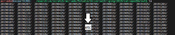
Some examples of what the shape of the directories would look like:
* The folder caliope20m, inside the sub-folder out, regarding the raw CALIOPE-Urban output for each day:
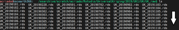
 * The folder UK1/UK/UK_raw/, where the corrections appear in terms of the day:
 * The folder UK1/images/, where the plots appear:
 Some plots after applying the methodology:
* Annual mean NO2 concentration from CALIOPE-urban:
ex6.pdf
* Annual mean NO2 concentration from the Universal Kriging correction:
ex7.pdf
* NO2 difference between CALIOPE-Urban and the Universal Kriging correction:
ex8.pdf
==== Universal Kriging using both covariates (adding the microscale-LUR basemap), the whole 2019 data and using the UK and cross applications ====
1. Preparing the configuration file, in this case is the following:
Some plots after applying the methodology:
* Annual mean NO2 concentration from CALIOPE-urban:
ex6.pdf
* Annual mean NO2 concentration from the Universal Kriging correction:
ex7.pdf
* NO2 difference between CALIOPE-Urban and the Universal Kriging correction:
ex8.pdf
==== Universal Kriging using both covariates (adding the microscale-LUR basemap), the whole 2019 data and using the UK and cross applications ====
1. Preparing the configuration file, in this case is the following:
 2. Enter to the machine
<code bash>
ssh bscXXXXX@nord4.bsc.es
</code>
3. Preparing the job, in this case we are going to reduce the number of cores and computational time, so change the queue too, and not require high memory.
<code bash>
#!/bin/bash
#SBATCH –job-name=“kriging_second”
#SBATCH –output=K_s_%j.out
#SBATCH –error=K_s_%j.err
#SBATCH –time=01:00:00
#SBATCH –qos=debug
#SBATCH -n 30
module load R
Rscript /esarchive/scratch/acriado/Rstudio/UniversalKriging/general/kriging_repository.R /esarchive/scratch/acriado/Rstudio/UniversalKriging/general/config_file.yml
</code>
4. Submitting the job.
<code bash>
sbatch kriging_repository.sh
</code>
5. Checking that everything is OK.
<code bash>
squeue
</code>
6. Waiting until the job is finished.
7. The job is completed. A folder named by UK2/ inside the folder 2019/ will be created, with the same folder structure presented above. Notice that as we have selected only 2 applications (UK and cross), the folders regarding the remaining ones will appear empty. In this case, new plots appear regarding the usage of the microscale-LUR basemap.
Some plots after applying the methodology:
* microscale-LUR basemap:
exc10.pdf
* Annual mean NO2 concentration from the Universal Kriging correction:
exc11.pdf
2. Enter to the machine
<code bash>
ssh bscXXXXX@nord4.bsc.es
</code>
3. Preparing the job, in this case we are going to reduce the number of cores and computational time, so change the queue too, and not require high memory.
<code bash>
#!/bin/bash
#SBATCH –job-name=“kriging_second”
#SBATCH –output=K_s_%j.out
#SBATCH –error=K_s_%j.err
#SBATCH –time=01:00:00
#SBATCH –qos=debug
#SBATCH -n 30
module load R
Rscript /esarchive/scratch/acriado/Rstudio/UniversalKriging/general/kriging_repository.R /esarchive/scratch/acriado/Rstudio/UniversalKriging/general/config_file.yml
</code>
4. Submitting the job.
<code bash>
sbatch kriging_repository.sh
</code>
5. Checking that everything is OK.
<code bash>
squeue
</code>
6. Waiting until the job is finished.
7. The job is completed. A folder named by UK2/ inside the folder 2019/ will be created, with the same folder structure presented above. Notice that as we have selected only 2 applications (UK and cross), the folders regarding the remaining ones will appear empty. In this case, new plots appear regarding the usage of the microscale-LUR basemap.
Some plots after applying the methodology:
* microscale-LUR basemap:
exc10.pdf
* Annual mean NO2 concentration from the Universal Kriging correction:
exc11.pdf